[2]:
import pandas as pd
import pyfas as fa
6. Tab files
A tab file contains thermodynamic properties pre-calculated by a thermodynamic simulator like PVTsim. It is good practice to analyze these text files before using them. Unfortunately there are several file layouts (
key, fixed, with just a fluid, etc.). The Tab class handles some (most?) of the possible cases but not necessarily all the combinations.The only public method is
extract_all and returns a pandas dataframe with the thenrmodynamic properties. At this moment in time the dtaframe obtained is not unique, it depends on the tab format and on the number of fluids in the original tab file. Room to improve here.6.1. Tab file loading
[14]:
tab_path = '../../pyfas/test/test_files/'
fname = '3P_single-fluid_key.tab'
tab = fa.Tab(tab_path+fname)
6.1.1. Extraction
[15]:
tab.export_all()
[16]:
tab.data
[16]:
| "1" | |
|---|---|
| CPG | [1898.12, 1905.92, 1913.71, 1921.51, 1929.3, 1... |
| CPHL | [1610.0, 1617.06, 1623.76, 1630.02, 1635.79, 1... |
| CPWT | [3454.74, 3458.93, 3463.33, 3467.94, 3472.76, ... |
| DROGDP | [8.4946e-06, 8.42111e-06, 8.34888e-06, 8.27788... |
| DROGDT | [-0.000323057, -0.000317492, -0.00031207, -0.0... |
| DROHLDP | [4.47091e-07, 4.5376e-07, 4.60533e-07, 4.67363... |
| DROHLDT | [-0.694011, -0.693068, -0.691885, -0.69043, -0... |
| DROWTDP | [5.24381e-07, 5.22483e-07, 5.1907e-07, 5.14565... |
| DROWTDT | [0.158913, 0.142489, 0.120409, 0.0942844, 0.06... |
| HG | [-19279.3, -14920.5, -10543.9, -6149.34, -1736... |
| HHL | [-317877.0, -313080.0, -308335.0, -303637.0, -... |
| HWT | [-1395510.0, -1387580.0, -1379650.0, -1371710.... |
| PT | [10000.0, 10000.0, 10000.0, 10000.0, 10000.0, ... |
| ROG | [0.0849146, 0.0841808, 0.0834595, 0.0827506, 0... |
| ROHL | [899.718, 900.424, 901.309, 902.434, 903.838, ... |
| ROWT | [813.363, 812.66, 811.929, 811.17, 810.382, 80... |
| RS | [0.999977, 0.999979, 0.99998, 0.999982, 0.9999... |
| RSW | [0.000692485, 0.000692485, 0.000692484, 0.0006... |
| SEG | [1185.33, 1201.82, 1218.24, 1234.58, 1250.85, ... |
| SEHL | [-587.526, -570.743, -554.118, -537.594, -521.... |
| SEWT | [-4115.44, -4085.47, -4055.71, -4026.17, -3996... |
| SIGGHL | [0.0280944, 0.0280288, 0.0279906, 0.0279847, 0... |
| SIGGWT | [0.0698809, 0.0690383, 0.0682086, 0.0673915, 0... |
| SIGHLWT | [0.0551154, 0.0550872, 0.0550879, 0.0551306, 0... |
| TCG | [0.0277744, 0.028032, 0.0282904, 0.0285496, 0.... |
| TCHL | [0.0969043, 0.0960938, 0.0953334, 0.094616, 0.... |
| TCWT | [0.548681, 0.553425, 0.558072, 0.562624, 0.567... |
| TM | [-10.0, -7.70833, -5.41667, -3.125, -0.833333,... |
| VISG | [1.01832e-05, 1.02634e-05, 1.03434e-05, 1.0423... |
| VISHL | [0.220481, 0.227562, 0.234135, 0.240676, 0.247... |
| VISWT | [0.0010661, 0.00101649, 0.000970794, 0.0009286... |
Some key info about the tab file are provided as tab.metadata
[17]:
tab.metadata
[17]:
{'fluids': [' "1"'],
 'nfluids': 1,
 'p_array': array([  1.00000000e+04,   1.01325000e+05,   7.38958000e+05,
          1.46792000e+06,   2.19688000e+06,   2.92583000e+06,
          3.65479000e+06,   4.38375000e+06,   5.11271000e+06,
          5.84167000e+06,   6.57063000e+06,   7.29958000e+06,
          8.02854000e+06,   8.75750000e+06,   9.48646000e+06,
          1.02154000e+07,   1.09444000e+07,   1.16733000e+07,
          1.24023000e+07,   1.31313000e+07,   1.38602000e+07,
          1.45892000e+07,   1.53181000e+07,   1.60471000e+07,
          1.67760000e+07,   1.75050000e+07,   1.82340000e+07,
          1.89629000e+07,   1.96919000e+07,   2.04208000e+07,
          2.11498000e+07,   2.18788000e+07,   2.26077000e+07,
          2.33367000e+07,   2.40656000e+07,   2.47946000e+07,
          2.55235000e+07,   2.62525000e+07,   2.69815000e+07,
          2.77104000e+07,   2.84394000e+07,   2.91683000e+07,
          2.98973000e+07,   3.06263000e+07,   3.13552000e+07,
          3.20842000e+07,   3.28131000e+07,   3.35421000e+07,
          3.42710000e+07,   3.50000000e+07]),
 'p_points': 50,
 'properties': ['PT',
  'TM',
  'ROG',
  'ROHL',
  'ROWT',
  'DROGDP',
  'DROHLDP',
  'DROWTDP',
  'DROGDT',
  'DROHLDT',
  'DROWTDT',
  'RS',
  'RSW',
  'VISG',
  'VISHL',
  'VISWT',
  'CPG',
  'CPHL',
  'CPWT',
  'HG',
  'HHL',
  'HWT',
  'TCG',
  'TCHL',
  'TCWT',
  'SIGGHL',
  'SIGGWT',
  'SIGHLWT',
  'SEG',
  'SEHL',
  'SEWT'],
 't_array': array([ -10.      ,   -7.70833 ,   -5.41667 ,   -3.125   ,   -0.833333,
           1.45833 ,    3.75    ,    6.04167 ,    8.33333 ,   10.625   ,
          12.9167  ,   15.2083  ,   15.56    ,   17.5     ,   19.7917  ,
          22.0833  ,   24.375   ,   26.6667  ,   28.9583  ,   31.25    ,
          33.5417  ,   35.8333  ,   38.125   ,   40.4167  ,   42.7083  ,
          45.      ,   47.2917  ,   49.5833  ,   51.875   ,   54.1667  ,
          56.4583  ,   58.75    ,   61.0417  ,   63.3333  ,   65.625   ,
          67.9167  ,   70.2083  ,   72.5     ,   74.7917  ,   77.0833  ,
          79.375   ,   81.6667  ,   83.9583  ,   86.25    ,   88.5417  ,
          90.8333  ,   93.125   ,   95.4167  ,   97.7083  ,  100.      ]),
 't_points': 50}
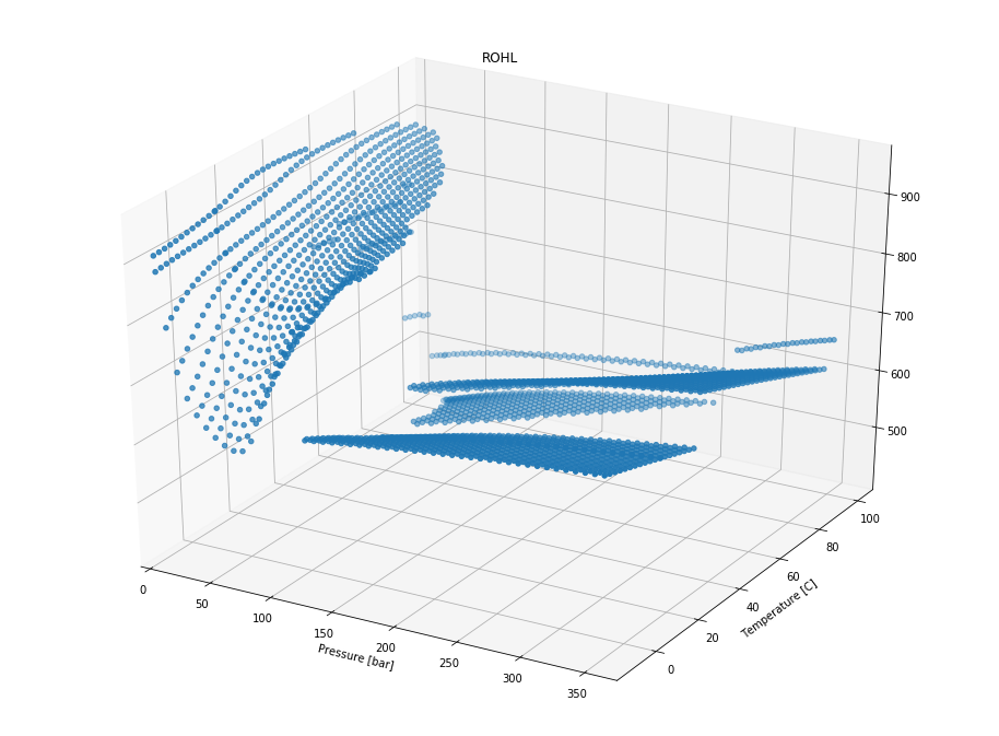
6.1.2. Plotting
Here under an example of a 3D plot of the liquid hydropcarbon viscosity
[48]:
import matplotlib.pyplot as plt
from mpl_toolkits.mplot3d import Axes3D
import itertools as it

def plot_property_keyword(pressure, temperature, thermo_property):
    fig = plt.figure(figsize=(16, 12))
    ax = fig.add_subplot(111, projection='3d')
    X = []
    Y = []
    for x, y in it.product(pressure, temperature):
        X.append(x/1e5)
        Y.append(y)
    ax.scatter(X, Y, thermo_property)
    ax.set_ylabel('Temperature [C]')
    ax.set_xlabel('Pressure [bar]')
    ax.set_xlim(0, )
    ax.set_title('ROHL')
    return fig
[49]:
plot_property_keyword(tab.metadata['p_array'],
                      tab.metadata['t_array'],
                      tab.data.T['ROHL'].values[0])
[49]:
[ ]: